Understanding Attention: The Idea Behind Modern AI
Back to blog

Understanding Attention: The Idea Behind Modern AI

Updated: Feb 6, 2026

One paper changed everything: Attention Is All You Need. This post breaks down the foundations behind attention, starting from embeddings. A simple journey from words to meaning.

Attention Mechanisms

I want to talk about attention.

The paper that changed everything.

The paper that gave birth to ChatGPT and forced the rest of the world to wake up.

“Attention Is All You Need.”

Today, we’re not going to talk about the entire Transformer architecture.

We’ll focus on attention.

But before we get there, we need to understand something fundamental:

embeddings.

Embeddings

When we talk to a language model like ChatGPT or Gemini, we use words.

That’s obvious.

But algorithms don’t work with words.

They work with numbers.

This is where embeddings come in.

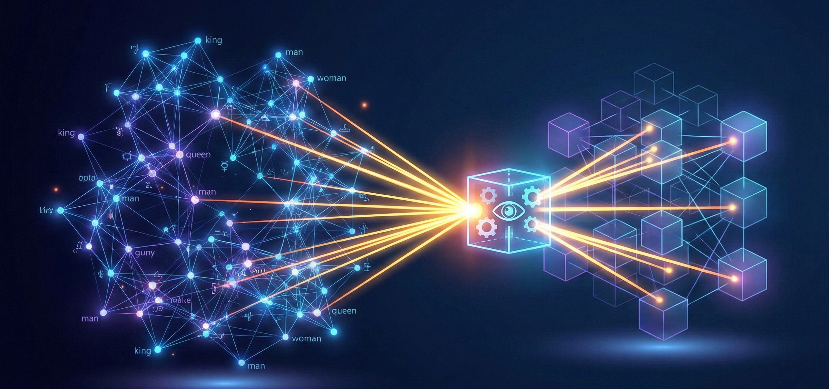
Embeddings are numerical representations of words inside a vector space.

Each word is mapped to a vector — a list of numbers — that captures meaning, context, and relationships with other words.

Words that mean similar things end up close together in that space.

And that leads to an important question:

What is a vector space?

A vector space is an algebraic structure defined over a set of elements where:

  • you can add elements together,

  • and scale them using numbers.

Formally speaking:

A vector space is an algebraic structure that arises when we define two internal operations and one external operation on a set of elements.

In the dropdown below, you can find the formal definition of a vector space (sorry, I just really love mathematics).

Let V be a non-empty set and let K be a field (typically or ).

We say that V is a vector space over K if the following operations are defined:

- Vector addition

- Scalar multiplication

and the following axioms hold for all and all .

Axioms of vector addition

Closure
For all

Commutativity

Associativity

Additive identity
There exists an element such that:

Additive inverse
For each , there exists an element such that:

So now, each word is represented inside a vector space that captures its meaning.

And something very powerful happens.

Once everything is expressed as vectors, we can add, subtract, scale, and combine them mathematically.

Even more importantly, metrics emerge.

That means we can measure distances between vectors.

We can compute similarities.

We can compare meanings.

For example, dog and cat are both animals, so the distance between their vectors will be small.

But the distance between cat and television will be much larger.

By giving words a vector structure, we unlock a whole new set of operations.

And this is where attention mechanisms come in.

This is the first step of large language models:
understanding the context surrounding a word.

Attention: Understanding Context

We already know that text can be turned into vector representations that encode meaning.

Well… “already know” is a bit generous, because we haven’t explained that transformation yet.

Quick preview: embeddings are produced by another model. I won’t spoil it now—we’ll cover that in a separate post.

So, assume each word/token is now a vector. Great.

Next challenge: capture how words relate to each other inside a sentence.

Example:

The elephant is very large.

Here, elephant should pay a lot of attention to large (it describes it), while is might matter less for this specific relation.

So how do we model that mathematically?

This is where the fun begins.

Get ready: we’re back to high-dimensional vector spaces and operations on them.

Let a token be represented as a vector:

where ddd is the embedding dimension (often hundreds or even thousands).

Now we apply linear projections to this vector.

The core idea is:

Instead of working directly in the full d-dimensional space, we project into smaller learned subspaces of size ​, where .

To do this, we use three learned matrices:

And compute:

These are called:

  • Query (q): what this token is looking for

  • Key (k): what this token offers / how it can be matched

  • Value (v): the information this token will pass on if selected

That’s the foundation of attention:

Tokens ask questions (queries), compare with others’ keys, and gather weighted information from their values.

What we are doing in the formula, multiplying by the weights , is projecting vectors onto learned subspaces.

For more information you can check the following deep dive.

These are linear transformations in algebra.

More precisely, each multiplication by a weight matrix maps the same token representation into a different feature space.

This does not simply scale numbers; it reorganizes information so different aspects of meaning become easier to separate and use.

What does each subspace represent?

When we project a token vector into , , and , we are not creating random vectors.

Each projection learns a different “view” of the same token.

You can think of it like this:

  • The original embedding : a rich, compressed meaning of the token.

  • The projections: specialized lenses for the attention mechanism.

1) Query subspace ()

This subspace represents what this token wants to find in other tokens.

If the token is “elephant”, its query might encode something like:

  • “I’m looking for attributes that describe me”

  • “I’m looking for words related to size, color, action, etc.”

So is an information request vector.

2) Key subspace (​)

This subspace represents what this token can offer to others.

A token’s key acts like a label or index:

  • “I contain useful information about being an adjective”

  • “I contain information about location/time/action”

During attention, other tokens compare their query with this key to decide:

“Is this token relevant for me right now?”

So is a matchability vector.

3) Value subspace (​)

This subspace represents the actual content to pass forward if the token is selected by attention.

Important distinction:

  • Key is for matching.

  • Value is for carrying information.

If attention weight is high, more of that token’s value is mixed into the output.

So is the payload vector.

By the way, one key point:

are trainable parameters (model weights).

They are not fixed by hand. During training, the model sees lots of data, makes predictions, measures error, and updates these matrices through gradient descent/backpropagation.

So over time, these weights learn:

  • how to build better queries (what to look for),

  • how to build better keys (how tokens should be matched),

  • and how to build better values (what information should be passed forward).

In short: the model learns from data how attention should work, by continuously adjusting ​, , and .

import math
import torch
import torch.nn as nn
import torch.nn.functional as F

class SelfAttention(nn.Module):
    """
    Minimal single-head self-attention implementation.

    Input shape:
        x: [batch_size, seq_len, d_model]

    Output shape:
        out: [batch_size, seq_len, d_model]
        attn_weights: [batch_size, seq_len, seq_len]
    """

    def __init__(self, d_model: int, d_k: int = None):
        super().__init__()
        # If d_k is not provided, use d_model (common in simple examples)
        self.d_model = d_model
        self.d_k = d_model if d_k is None else d_k

        # Trainable projection matrices:
        # W_q, W_k, W_v are implemented as Linear layers.
        # They map each token embedding from d_model -> d_k (for q, k)
        # and d_model -> d_model (for v in this simple version).
        self.W_q = nn.Linear(d_model, self.d_k, bias=False)
        self.W_k = nn.Linear(d_model, self.d_k, bias=False)
        self.W_v = nn.Linear(d_model, d_model, bias=False)

    def forward(self, x: torch.Tensor, mask: torch.Tensor = None):
        """
        x: [B, T, D]
        mask (optional): [B, T, T] with 1 for allowed positions, 0 for blocked positions
                         (useful for padding mask or causal mask)

        Returns:
            out: [B, T, D]
            attn_weights: [B, T, T]
        """
        # 1) Project input embeddings into Query, Key, Value subspaces
        # q: [B, T, d_k], k: [B, T, d_k], v: [B, T, D]
        q = self.W_q(x)
        k = self.W_k(x)
        v = self.W_v(x)

        # 2) Compute raw attention scores with dot product q @ k^T
        # scores shape: [B, T, T]
        # Each position i compares its query q_i with every key k_j.
        scores = torch.matmul(q, k.transpose(-2, -1))

        # 3) Scale scores to stabilize training
        # Without scaling, dot products can grow too large for big d_k.
        scores = scores / math.sqrt(self.d_k)

        # 4) (Optional) Apply mask
        # Positions with mask == 0 are set to a large negative value,
        # so after softmax they become ~0 attention probability.
        if mask is not None:
            scores = scores.masked_fill(mask == 0, float("-inf"))

        # 5) Convert scores into probabilities with softmax
        # attn_weights[b, i, j] = how much token i attends to token j
        attn_weights = F.softmax(scores, dim=-1)

        # 6) Weighted sum of values
        # out_i = sum_j attn_weights[i, j] * v_j
        # out shape: [B, T, D]
        out = torch.matmul(attn_weights, v)

        return out, attn_weights


if __name__ == "__main__":
    # Reproducibility
    torch.manual_seed(42)

    # Example dimensions
    B = 2          # batch size
    T = 5          # sequence length
    D = 16         # embedding size
    d_k = 8        # query/key subspace size

    # Dummy token embeddings
    x = torch.randn(B, T, D)

    # Create attention module
    attn = SelfAttention(d_model=D, d_k=d_k)

    # Forward pass
    out, weights = attn(x)

    print("Input shape:   ", x.shape)        # [2, 5, 16]
    print("Output shape:  ", out.shape)      # [2, 5, 16]
    print("Weights shape: ", weights.shape)  # [2, 5, 5]

    # Optional: inspect attention of first batch item
    print("\nAttention matrix for sample 0:")
    print(weights[0])

Let’s Dig Deeper into Attention

At this point, we know that Transformers learn projection weights to compute attention.
Now the key question is: how is attention written mathematically?

The core formula is:

Because embeddings are vectors, we can compare them numerically.

Breaking down the formula

  1. Compute similarity scores

Each entry measures how much token (as a query) matches token (as a key).

  1. Scale the scores

Without scaling, dot products can grow large when is large, making softmax too peaky and gradients unstable.

  1. Normalize with softmax (row-wise)

This gives attention weights :

  • each weight is in ,

  • each row sums to ,

  • larger scores get larger weights.

  1. Weighted sum of values

For each token , the output is a weighted combination of all value vectors .
So token “looks more” at tokens with higher attention weights.

Why do we need softmax?

Without softmax, scores are unbounded raw numbers (negative, positive, any scale).
With softmax, they become a clean probability-like distribution over tokens:

  • Easy to interpret (“how much attention goes to each token”)

  • Comparable across positions

  • Differentiable and stable for training.

1) What are Q, K, and V?

For each token representation xix_ixi​, the model computes:

  • (query): what this token is looking for.

  • (key): what this token offers.

  • (value): the content this token contributes if attended.

2) Why dot product?

The compatibility score between token iii and token jjj is:

Dot product can be written as:

So it measures alignment:

  • large positive similar direction high compatibility,

  • near zero weak relation,

  • negative opposite direction.

That is why is interpreted as “how well they match.”

3) Why does appear?

If we stack all queries and keys:

then:

and each entry is:

So one matrix multiplication computes all pairwise query-key scores at once.

4) Short linguistic intuition

In the sentence:
“The cat ate fish because it was hungry.”

the query for “it” may align more with “cat” than with “fish,” so the score for “cat” is higher, and attention puts more weight there.

Test Your Knowledge

Take this quiz to test your understanding of the concepts covered in this article.

15 questions • ~23 min

Share this article